
Eaqan Chaudhry, Salisbury University
Introduction
All writing centers strive towards a common goal: to help students become better writers – regardless of the particular assignment or stage of the writing process in which the writer arrives at the writing center. Driscoll & Perdue (2014) have expressed the need for and importance of more RAD (replicable, aggregable, and data-supported) research within writing centers in order to construct evidence-based practices to expand upon the services provided by writing centers as a whole. Several studies have highlighted the benefits of RAD-based research. For instance, Giaimo (2017) employed such assessments to evaluate student learning within writing centers and the specific conditions under which learning and development can occur effectively. RAD research is particularly important for understanding why students choose to use writing centers and how centers can then develop student-centered services. This need for writing center services that better align with student needs is emphasized by Denny, Nordlof and Salem (2018) when drawing attention to the disparity between student perceptions of writing centers and how writing centers perceive themselves. Salem (2016) has taken this a step further by arguing that writing centers can be more than merely areas in which students can work on their assignments in a peer-to-peer setting; rather, these institutions can aim to better serve their respective campus communities in a more comprehensive manner. I propose that centers could do this by evaluating trends among student concerns and how they are shaped by contexts beyond those Salem (2016) examines (i.e.: SAT scores, race, gender, native language, etc.).
Salem’s study was foundational for understanding the relationship between demographic variables and writing center usage, and this study proposes the use of statistical analyses to further understand this relationship by expanding the categories of consideration from demographic information to include contextual factors as well. This can help us identify similarities and trends among students who take advantage of the services writing centers provide. But such information is limited in that it would merely tell us which students are visiting, while neglecting to consider the broader variables surrounding the context of student visits. Although we as writing center staff may often think of these sessions as occurring within a vacuum, there are external variables at play. In addition to the variables studied by Salem, contextual variables I noticed could impact session focus included: class year, assignment due date, whether the assignment was for a class within the student’s major (defined as “within major”), whether the student was an international student, and whether it was their first time visiting the writing center. These are just some of the external factors at play when a student visits the writing center, and although the extent to which they affect the session focus (the aspects of their writing on which a student wishes to focus during a session) may vary, we may be able to elucidate the interactions between the aforementioned factors in order to identify trends within institutions, and subsequently use those trends to inform any decisions regarding major changes pertaining to expanding writing center services and comprehensively addressing what students will need in order to improve themselves as writers.
This paper explores the use of two statistical methods that can be used within writing centers and it will serve as a methodological guide so practitioners can use these methods to conduct similar analyses at their own institutions with the goal of gaining insights into broader trends pertaining to writing concerns among their campus communities. This paper will first provide more detail about our local context, background, and an explanation of the two statistical models used; it will then delve into in-depth methods for using the models within Program R so other institutions can replicate our methods for their own studies and purposes.
Study Contexts
At the Salisbury University Writing Center (Salisbury, MD, USA), we aim to expand upon writing center practices by developing tailored workshops to target common writing concerns among our campus community. However, in order to do so, we must first identify the general trends in writing concerns from those students visiting the writing center. We addressed this by employing two statistical methods – Multiple Correspondence Analysis and Path Analysis – to evaluate the writing concerns students wish to address during a session, and how these concerns are shaped by contexts such as the students’ class year, assignment due dates, and additional factors. We selected these analyses as they would allow us to reduce the number of variables being analyzed into fewer and broader terms, and discern both direct and indirect relationships between contextual factors and the aforementioned variables., in order to provide a more comprehensive insight into students’ writing concerns in our own center. We are utilizing a novel approach to expanding upon writing center practices as the use of these methodologies and their broader implications has yet to be explored in writing center research. The goal of this paper is to describe and guide the reader through the steps involved in conducting two statistical analyses necessary for evaluating statistical significance and visualizing how writing concerns are shaped by contexts that expand upon Salem’s study. We hope explaining our methods of analysis will allow other centers with contexts that differ from our own to conduct similar analyses to identify and address trends in students’ writing concerns.
Two Statistical Models to Analyze Writing Center Usage Trends
Path Analysis
One method through which the interactions between these factors can be explored is a path analysis, which is a form of multiple regression statistical analysis that evaluates causal models by looking at the magnitude and direction of significant interactions between a dependent (response) variable and one or more independent (predictor) variables . In other words, it is a flow chart that designates arrows to display the statistically significant effects of a predictor variable on a response variable. The added benefit of using a path analysis over other statistical analyses is that not only are we able to see the direct significant interactions between the independent and dependent variables, but we are also able to visualize any potential indirect effects that may only occur when a third variable is present as a mediator. So in the context of a writing center, we would use student demographic information as independent variables while the variables associated with session focus would be considered dependent variables. This would be due to the fact that any changes in the session focus would depend on variation in the demographic information, thus establishing session focus as the dependent (or response) variable, whereas the demographic characteristics are unaffected by the session focus. For example, a student’s propensity to work on their thesis statement may not affect their class year, however, the reverse may be a valid relationship, where they may be more likely to work on their thesis statement if they are a junior. However, since the dependent (response) variable here is the session focus, which likely includes many (~10) variables, a path analysis with this set of variables would be far too convoluted and we would have trouble parsing out the truly important significant interactions.
Multiple Correspondence Analysis (MCA)
To ameliorate this concern, we can use another statistical method known as Multiple Correspondence Analysis (MCA) in order to first “condense” many variables into fewer broad variables which accurately represent the original data set. These broad variables can then be incorporated in the path analysis. The purpose of condensing these multiple variables is to parse out the underlying trends occurring within our data set. If we were to analyze ten dependent variables with 5 independent variables, there are 50 potential relationships, of which many could be significant. If this is the case, the plethora of significant relationships would only muddle the picture, as we are focusing on larger trends such as the effect of class year on stage of the writing process, rather than very specific interactions (such as the effect of class year on thesis statement alone) which could potentially limit the broader applications of our findings. Such larger trends can tell us more in terms of how the contexts surrounding writing are affecting session focus, and how our findings can be applied in a practical context. MCA is a form of correspondence analysis which can be applied to qualitative (categorized) data, where underlying patterns within the data set can be identified and displayed in a low-dimensional geometric space. For example, an MCA can be used to “condense” ten variables into two variables (D1 and D2, respectively), which are subsequently termed dimensions. These dimensions can then be used to explain a certain percentage of variability within the data set; the MCA also assigns a scaled number for each individual sample/session within each dimension. So continuing with the earlier example, if D1 explains approximately 21.99% of the variability within the data set, and D2 explains 17.73% of the variability within the data set, these two dimensions together explain 39.72% of the variability within the data set (Figure 1).
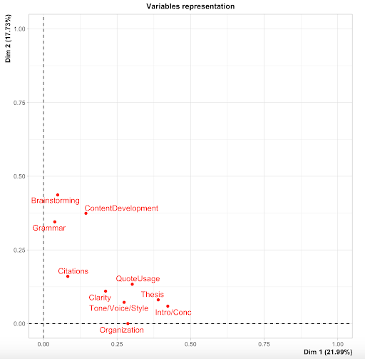
Furthermore, these dimensions also represent the ten variables we initially began with, meaning that D1 would predominantly represent thesis statement and grammar. This would indicate that sessions associated with a higher number on the D1 scale involved students wanting to work on thesis statement and grammar, while those associated with a lower number on the D1 scale were less likely to want to work on thesis statement and grammar. This is then expanded into the number of dimensions being considered in the final analysis.
Generally, this correspondence analysis is helpful in looking at broad patterns among students and usage of the writing center and the factors that influence this usage. My goals here are to describe how both of these analyses can be conducted in Program R (a free statistical computing software) by providing steps for those who may be unfamiliar with coding or statistical analyses. Ultimately this methodology has broad applications, and can primarily be utilized by writing centers to evaluate how the contexts surrounding their writing are affecting what writers wish to focus on during a session, and how we can use our knowledge of these interactions to better address student concerns while fostering better writing practices across campuses.
Methods
Study Design and Sampling Techniques
WCOnline is a scheduling and recordkeeping program that has become popular among writing centers – including the Salisbury University Writing Center. This program allows students to set up appointments online. In doing so, writing centers are able to collect some demographic information about each session/writer, such as the due date for the assignment, whether they are visiting the writing center for the first time, and the session focus (i.e. brainstorming, content development, introduction/conclusion, thesis statement, organization, clarity, tone/voice/style, grammar, quote usage, and citations) all of which are self-reported by the writer when setting up the appointment. Because WCOnline is utilized among many writing centers, the data we have chosen to collect is customizable and can be tailored to individual center needs – meaning that no extraneous data collection (outside of WCOnline) is necessary to conduct the analyses outlined in this paper. At the Salisbury University Writing Center, we used WCOnline to obtain self-reported demographic information, such as the students’ class year, their major, first language, and whether they were an international student.
As this was a quantitative study using statistical regression and pathway analyses, we needed to define our predictor (independent) and response (dependent) variables. The contextual predictor variables we analyzed included: class year, assignment due date, whether the assignment was for a class within the student’s major (defined as “within major”), whether the student was an international student, and whether it was their first time visiting the writing center. The session focus (our response variables) being analyzed included aspects and stages of their writing for which students arrived at our writing center: brainstorming, content development, introduction/conclusion, thesis statement, organization, clarity, tone/voice/style, grammar, quote usage, and citations. As described above, session focus data was collected over the course of two years from self-reported questionnaires which students completed prior to making an appointment. These questionnaires inquired the aspects of their writing upon which students wanted to focus during a given session. We selected these specific variables, as they provided us with information about the contexts surrounding both the writer (e.g. class year, whether they were an international student) and the writing assignment (e.g. due date, whether it was for a class within their major).
In our study, any data pertaining to demographic information was deidentified prior to statistical analysis in the interest of the privacy of the students and in order to comply with FERPA and IRB guidelines. In addition, because much of our data consists of categorical variables (i.e.: class year is either freshman, sophomore, junior, or senior; whether they wanted to work on their thesis statement is either yes or no) and some statistical programs could potentially encounter issues when processing text inputs as variables[1] , we coded our data for these categorical responses in order to streamline the data analysis. This was done by assigning a numerical value to each response (i.e. yes = 1 and no = 2).
This study collected data spanning from August of 2017 to January of 2020, providing us with data from a total of 5,193 writing sessions. Students were allowed to schedule multiple appointments, and if students scheduled multiple appointments over the course of this study, the appointment was classified as either their first visit or a returning visit. Our timeline allowed us to analyze data collected throughout multiple semesters, which accounted for fluctuations in writing center visits throughout the academic year. Additionally, it allowed us to have a large enough sample size to be representative of our campus population. Consequently, the results of this study allowed us to draw inferences regarding the needs of writers within our campus community. Since there are differences between various types and sizes of writing centers, as well as the universities and communities in which they are housed, we propose that the methods described here can be replicated at other institutions so writing centers can expand and tailor their services to better serve the needs of their campus communities.
Data Collection and Analysis
Multiple Correspondence Analysis
Prior to starting the data analysis, it is imperative to ensure the data set has been imported into Program R via the “Import dataset” in the Environment window on the top right. The window on the bottom right can serve to view files, plots/graphs, download packages necessary to conduct certain analyses, and help menu (which can be used to identify the purpose of any command by simply typing the command [the text preceding the parentheses in each line of code] into the search query). All of the lines of code described in this paper will be entered in the window on the top left. When each line of code is run (which can be done by highlighting the text you wish to run and clicking “Run” on the top right corner of the terminal; another way to do this is to click on the line of code, and pressing Ctrl/Cmd+Enter on the keyboard), the corresponding outputs should appear in the console (on the bottom left). Note that any text following a “#” symbol is not incorporated into the output and will appear as green text in the console, so this can be used to add notes within the code as seen below. For our analysis, “UWCF17W20” served as a placeholder referring to the data set (the actual text in place of UWCF17W20 is up to the discretion of the practitioner working with the data set).
##Start here
View(UWCF17W20)
names(UWCF17W20)
str(UWCF17W20)
options(max.print=1000000) ## this sets upper limit for sample size
print(UWCF17W20)
The above text will open the file with the data set and provide descriptive statistics. The View command will prompt Program R to open and view the imported data set.
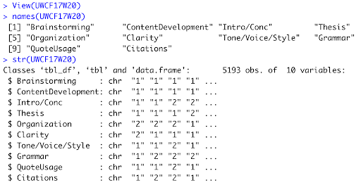
The Names command will display the names of all variables; Str will display the structure of the data set by listing the names of the variables, their classification (continuous scale variables or categorical character variables – in the case of our data set, the latter), sample responses for each variable, and the total sample size of the data set (Figure 2). These commands are necessary to ensure that the data set has been properly imported, that there are no formatting errors, and that the variables have been classified (as continuous/numeric or categorial/characters) properly. A sample output of these commands is seen in Figure 2. Before proceeding, we must consider that last component: the sample size of the data set. Program R sets an arbitrary limit of sample sizes to display, which, if left unchecked has the potential to severely limit the power of the analyses. Researchers can rectify this by setting an upper limit of samples that we want Program R to read and display, which can be accomplished through the options(max.print=???) command. Researchers can either set the upper limit slightly above their sample size, or make it an extraordinary large number (like 1000000) so they do not have to worry about it for the foreseeable future (unless, of course, your writing center reaches one million sessions, in which case, congratulations!). Another caveat to mention here is that numerical values entered in Program R do not need a comma (so the proper syntax for one million would be 1000000, not 1,000,000). The print command will then display your entire data set in the console window.
To begin the actual analyses, there are some packages that will need to be installed. In Program R, packages are defined as a fundamental unit of sharable code, for which we can use defined commands to expedite the process for data analysis. Typically some commands are specific to a package; thus they cannot be used (and will return an error message) if entered without installing and opening the necessary package first. This can be done one of two ways: begin by navigating to the window on the bottom right, select the “Packages” tab, click install, and type in the names of the packages within quotations in the code below (e.g. FactoMineR); a more efficient method would be to type in the commands to have R download the packages itself. For the latter, see below:
install.packages (“FactoMineR”)
install.packages (“ggplot2”)
install.packages (“factoextra”)
install.packages (lavaan)
install.packages (semPlot)
install.packages (OpenMx)
install.packages (tidyverse)
install.packages (knitr)
install.packages (kableExtra)
install.packages (GGally)
The first three packages will be able to carry out commands necessary for the Multiple Correspondence Analysis, while the remainder of the packages will be necessary for the Path Analysis. Upon installing the aforementioned packages, the researchers must enter the library command, which will pull the indicated package R to load these packages. So in the case of the library(“FactoMineR”) command, R will pull the FactorMineR package from its library, which will allow the researchers to use commands (which are specific to that package) to conduct the analysis with our data set. It is imperative to include library command, because if we neglect to do so, Program R will not recognize certain commands, even if they are typed correctly.
library(“FactoMineR”)
library(“ggplot2”)
library(“factoextra”)
summary(UWCF17W20)[, 1:10]
The summary command will provide a summary of the data set, with sample sizes and classifications of each variable. This may seem redundant, given that it was also done prior to installing the packages, but this command is included here to ensure that R is still reading the data set properly. We can control which variables are included in the summary (and later in the analysis) by listing within brackets the range of column numbers for which we are requesting a summary. For instance, if researchers are examining the 10 variables in the first 10 columns of a data set, the summary command would be followed by [, 1:10] to indicate columns/variables 1-10. The next command will carry out multiple processes concurrently.
mcaoutput <- MCA(UWCF17W20, ncp = 10, graph = TRUE)
The MCA command will conduct the actual Multiple Correspondence Analysis, while the information in the parentheses will provide the details of this analysis; first the researchers must enter the name of the data set (in our case, UWCF17W20). Next, ncp allows us to define the number of dimensions we intend to keep in the results; for this analysis, we chose to keep 10 dimensions (even though we likely won’t use more than 2-3 dimensions – since it is difficult to visualize results in any dimension past the third dimension) so we can see the relative contribution of each dimension to the variability of our data. Additionally, graph determines whether a graph is displayed ( = True prompts the program to display a 2-dimensional graph, similar to the one depicted in Figure 1, while = False will tell the program not to display a graph). Separate packages and lines of code may be necessary to display a 3-dimensional graph. Finally, any arrow pointing to the left allows us to name a variable or command. In our case, we defined the results of the Multiple Correspondence Analysis as mcaoutput, which is useful for our next command. The caveat with this command is that, while it conducts the MCA and provides a 2-D graph, it doesn’t display the actual results of the MCA.
Our final command for the MCA is as follows:
summary(mcaoutput, ncp = 3, nbelements = Inf)
This provides a summary of the MCA results, as seen in Figure 3. The first part of our output shows the percentage of variance in the data explained by each dimension. Following this output, R will provide an output assigning a score for each individual sample within each of the assigned dimensions (ncp=3 in the last command). These values can be exported (or copied and pasted) to Excel; they will be relevant for the path analysis. The third portion of this output will display how each of the initial variables score on the axes of each assigned dimension (Figure 4). Unfortunately, we cannot use all provided dimensions, as this would be difficult to visualize and defeat the purpose of the MCA (to “condense” the initial variables with which we began the analysis into fewer, more powerful dimensions which represent underlying trends in the data set). Next, we must examine the MCA output to see which variables have comparatively higher scores within each dimension. The last part of the MCA involves establishing which variables are heavily loaded in each dimension, then establishing a name for that dimension based on the session focus variables that respective dimension represents.
Path Analysis
It is imperative to remember the distinction between the purposes of statistical analyses like an Analysis of Variance (a test used to evaluate differences among group means in a sample) as compared to a path analysis: the former can be used to look at the direct significant effects of multiple independent variables on dependent variables, whereas the latter can elucidate both direct and indirect interactions.
To set up the path analysis, we must copy and paste the scores for the individual samples within each assigned dimension (the second portion of the MCA output) to the Excel file with our original data sheet. Next, we will rename and import the Excel file (in our study, we named this new file “UWCforPA”) with the addition of these assigned dimension values to Program R. We must then set up commands similar to those in the beginning of the MCA in order for Program R to view the file and subsequently provide descriptive statistics (recall that any text following the “#” symbol is not incorporated into the output, but is rather kept as a comment):
##Path Analysis starts here
View(UWCforPA)
names(UWCforPA)
str(UWCforPA)
options(max.print=1000000) ## this sets upper limit for sample size
print(UWCforPA)
summary(UWCforPA)
The library command will then be used to load the packages we’ll need for the path analysis:
library(lavaan)
library(semPlot)
library(OpenMx)
library(tidyverse)
library(knitr)
library(kableExtra)
library(GGally)
At this point, researchers can begin using the variables to set up the models for the path analysis. The first step in setting up these models entails defining the model parameters, which can be achieved by listing the dependent variables first, followed by the independent variables, all within single quotations. These quotations will set the boundaries of our model within the code. The dependent variables here (MC1, MC2, and MC3) are listed first with a “+” symbol in between each variable to group the dependent variables together, and the independent variable is included after the tilde (“~” symbol) which defines it as the predictor/independent variable. Moving forward, keep in mind that any variable(s) preceded by the tilde will be the independent variable(s):
model.focus<-‘
MC1 + MC2 + MC3 ~ ClassYear
‘
The first line shown here is naming this model “model.focus,” whereby the model explains the effects of Class Year on MC1, MC2, and MC3 (middle, early, and late-stage writing, respectively). Upon setting up the model, the next command will conduct the path analysis.
fit <- sem(model.focus, data = UWCforPA)
The sem command carries out the path analysis (sem stands for structural equation modelling – of which path analysis is a variation). But, similar to the mcaoutput command earlier, this does not visualize the results. In order to do so, we must label the path analysis (labelled in the sample analysis above as “fit”). We can then see a summary of the path analysis output by running the commands below:
summary(fit)
summary(fit, standardized = T, fit.measures = T, rsq = T)
The first command will provide a summary of the raw output, while the second command displays standardized values, which will be the ones used in the interpretation of the data. In addition, the second command can also provide r-squared values to show us how well the data fits the regressions. Within the path analysis output, the p-value for the regressions will indicate the statistical significance of the interactions between the demographic variables and MCA dimensions (statistical significance is achieved when p < 0.05), while the β coefficient denotes the direction and magnitude of these interactions.
A complete model looking at all direct effects for the data set would include all independent variables (the demographic information that researchers collected) and dependent variables (the three MCA dimensions being incorporating into the analysis). So the commands to set up a sample model for this complete data set would be as follows:
model.focus2<-‘
MC1 + MC2 + MC3 ~ ClassYear + WithinMajor + International + DueDate + FirstVisitBinary
‘
fit.2 <- sem(model.focus3, data = UWCforPA)
summary(fit.2)
summary(fit.2, standardized = T, fit.measures = T, rsq = T)
Again, the actual labels of these variables (i.e. model.focus2 or fit.2) are arbitrary and entirely up to the discretion of the researcher (they can be named “model.avocado” for all it matters).
semPaths(fit.3,’std’,layout=’tree2′)
At this point, we can visualize the output of the path analysis by entering the final command, seen above. As long as the semplot package has been loaded (per the library(semplot) command on page 10), the semPaths command will be able to produce a path analysis graph (Figure 6) in the “plots” tab in the window on the bottom right.
To look at indirect effects, we must create individual models for all possible indirect interactions, whereby we specify the predictor variable, response variable, and mediator. The total number of possible indirect effects will depend on the number of variables being examined. For instance, to examine whether there is a significant indirect effect of WithinMajor on MC2 with ClassYear as a mediator, one must set up the following model:
INDIRECT EFFECTS of WithinMajor –> ClassYear –>
MC2######
modelind1 <- ‘
##direct effect##
MC2 ~ c*WithinMajor
mediator##
ClassYear ~ aWithinMajor
MC2 ~ bClassYear
indirect effect(ab)##
ab := ab
total effect##
total := c + (a*b)
‘
fitind1 <- cfa(modelind1, data=UWCforPA)
summary(fitind1, standardized=TRUE)
tofit.modelind1 <- sem(modelind1, UWCforPA)
summary(tofit.modelind1, fit.measures = TRUE)
semPlotModel(fitind1, ‘std’, ‘est’, curveAdjacent = TRUE, style = “lisrel”)
Path diagram##
semPaths(fitind1, ‘std’, layout = ‘circle’)
Firstly, the text within the # symbols serves to specify the interactions being examined, which is useful if researchers are setting up multiple models simultaneously. The first modelind1 <— ‘ command designates a name for this model, and the specifications of the model are listed between two apostrophes. To set up the model, we must first assign letters to each effect; these letters will later be used as variables in the equation for indirect effects. If we are examining the effect of WithinMajor on MC2 with ClassYear as a mediator, the direct effect of WithinMajor on MC2 is first assigned the letter “c” (as seen in the MC2 ~ cWithinMajor command). Next, we can examine the indirect effect with ClassYear as a mediator by assigning the letter “a” to the effect of WithinMajor on ClassYear, and “b” to the effect of ClassYear on MC2. This is then specified as an indirect effect in the ab := ab command. Lastly, the total := c + (ab) command sets up the total effect: both the direct effect of WithinMajor on MC2 (c), and the indirect effect where ClassYear is a mediator (ab). The final apostrophe below this command indicates that we have finished defining the model. The fitind1 command will run the model and label the results, and the summary command will provide the p-values and β coefficients (labelled “estimates in the output”) of the interactions. This process can then be repeated for all possible indirect interactions.
We have now conducted a path analysis which examines both the direct and indirect effects between our independent and dependent variables. The magnitude and direction of these effects will be denoted by green and/or red lines, which represent positive and negative effects, respectively (based on the β coefficient values, which are also shown in the diagram).
Results
Multiple Correspondence Analysis
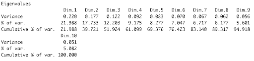
Based on the summary of the MCA results (Figure 3), we can extrapolate that the first three dimensions cumulatively explain approximately 51.924% of the variance in our data.
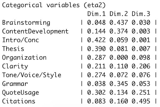
When examining the relative weight of the dependent variables (Figure 4), we established an arbitrarily assigned cutoff point of 0.200, whereby any values below this number were considered not “heavily loaded,” or in other words, not comprising a large portion of that dimension. Our results indicated that Introduction/Conclusion, Thesis statement, and Organization were more “heavily loaded” within Dimension 1 because they had the highest values in that column, meaning that Dimension 1 was most representative of those three variables. In our case, Dimension 2 was heavily loaded with Brainstorming, Content Development, and Grammar – all of which entail the first steps in writing a paper: brainstorming ideas for a thesis statement, main claims, and supporting information. Dimension 3 was heavily loaded with Clarity and Citations, which represent the “finishing touches” in the writing process when writers want to review their assignment to ensure it makes sense and their citations are properly formatted. Dimension 1, described earlier, is associated with Introduction/Conclusion, Thesis statement, and Organization, which compared to Dimensions 2 and 3, would be closer to the middle of the writing process – after brainstorming and developing ideas, and prior to checking for clarity and citations (as most writers ensure that the content of their paper is close to completion prior to making finishing touches to clarity and citation format). As a result, Dimensions 1-3 could be defined as middle-stage writing, early-stage writing, and final-stage writing, respectively. The naming of these dimensions is entirely dependent upon which variables are heavily loaded in each dimension, and this may vary from one writing center to the next. The findings of the Multiple Correspondence Analysis indicated that we successfully “condense” the variables we were analyzing to allow for broader analysis.
Path Analysis
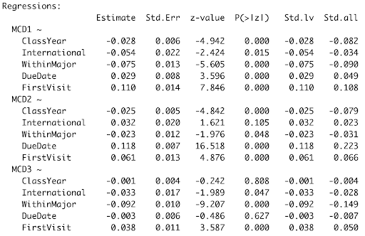
The results of the regression analyses are depicted in the output in Figure 5, and the statistically significant relationships are visualized in the path analysis diagram (Figure 6).
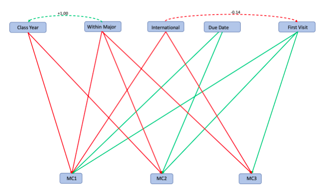
The results of our path analysis indicated that Class Year had a significant negative effect on whether writers wanted to address the concerns represented by MC1 and MC2 (mid-stage writing and early-stage writing, respectively). The negative effect of Within Major on MC1, MC2 and MC3 indicates that students were less likely to arrive at the writing center with assignments for classes within their major. In other words, they most often arrived with assignments for classes outside their major. However, the picture becomes more complex when considering indirect effects. Within Major was positively correlated with Class Year, indicating an indirect positive effect of Within Major on MC2 when considering Class Year as a mediator. First Visit had the opposite effect, indicating that students are more likely to focus on MC1, MC2 and MC3 if they are visiting the writing center for the first time. This may seem intuitive, as students visiting the writing center may entail exploring all aspects of their writing to pinpoint strengths and weaknesses.
A writer’s status as an international student negatively affected the likelihood that they would want to focus on MC1 and MC3 (mid-stage and final-stage writing concerns) during a session. Lastly, the time between the writing session and the assignment due date positively affected the likelihood that the writer would want to work on MC1 and MC2 (mid-stage and early-stage writing concerns, respectively). Furthermore, the β coefficients associated with these relationships suggest that the positive effect of Due Date is of greater on MC2 (early-stage writing; β = 0.118) than MC3 (mid-stage writing; β = 0.029) (Figure 5).
Discussion
The significant impact of Class Year on MC1 and MC2 suggests that as students progress in their academic careers, their writing concerns shift, and they are less likely to want to work on early-stage and mid-stage writing concerns. This in and of itself is intriguing, but it becomes even more compelling when considering the indirect effect of whether the assignment with which they arrive at the writing center is for a class within their major. The positive correlation between Within Major and Class Year indicates that despite both variables having a negative effect on MC2, Within Major may have a positive indirect effect on MC2 when Class Year is present as a mediator. This expands upon our previous interpretation about the effect of Class Year on MC2 by positing that as students progress in their academic careers, they are less likely to want to work on early stage writing – unless the assignment is for a class within their major, in which case they are more likely to want to work on early-stage writing. The positive effect of Due Date on MC1 and MC2 suggests that the earlier from a due date a student arrives at the writing center, the more likely they will focus on early-stage writing and mid-stage writing, with a preference towards early-stage writing with a greater time between the writing session and assignment due date. This finding supports the sentiment that when working on a writing assignment, it is best to start early and write often, as that will allow writers to receive effective feedback from writing centers if they so choose. The negative impact of International Student status on MC1 suggests that international students are less likely to want to focus on mid-stage writing concerns during a session, as compared to early-stage (brainstorming content development grammar) and final-stage writing (clarity and citations).
In the case of Salisbury University, these findings highlight the potential for tailored workshops to better serve the campus community. For instance, the increased propensity of students at Salisbury University to emphasize early-stage writing within their field as they progress in their academic journey may be indicative of a need to focus on how to approach professional writing within other fields. We could ameliorate this concern by developing workshops that review the general tenets of topics such as scientific writing and personal statements. Similarly, we could develop workshops tailored addressing early-stage writing concerns (brainstorming, content development, and grammar) for international students, as we found they were least likely to want to focus on mid-stage and final-stage writing concerns. Generally, these findings allow us to better identify the needs of writers within our campus community by providing us with insights pertaining to which aspects of writing certain demographics do and do not want to focus on during a session. In identifying these trends, writing centers can expand their roles in order to more effectively and holistically foster better writing practices. Certainly, workshops are not the only method of addressing these underlying trends in student writing concerns. Writing center practitioners can and should utilize creative practices to develop myriad techniques through which they could address these concerns.
The implications of the results obtained from such analyses should not be taken lightly, as not only do these findings provide us with information about the manner in which outside factors are influencing whether a student chooses to take advantage of the services provided by the writing center, but they also make us cognizant of the specific aspects of writing on which students wish to focus during a session. Furthermore, these analyses allow us to see the interplay between some of the aforementioned external variables, and how the writer’s time and concerns are prioritized in the context of the session. We can use this information to better serve campus communities by considering the impact of such contexts when attempting to foster better writing practices. Our results were particular to the campus community at Salisbury University, but the framework for this analysis – the code included – can be applied to any data set for writing centers at any other institution. We hope that other writing centers take advantage of the code included here, which will only require them to import their own data set and conduct this analysis with data from their own institution. The framework described here can allow writing centers to examine trends at the institutional level, the state level, the regional level, and even the international level. Being able to identify these trends in writing center usage and session focus may allow writing centers to effectively address student concerns while encouraging better writing practices across campuses.
Keeping the overarching goal of writing centers – helping students become better writers – in mind, along with Salem’s call for writing centers to do more outside of solely peer-to-peer sessions, we can see that the broader applications of such research is myriad. Because this type of analysis can allow writing centers to learn more about the contexts surrounding student visits and be cognizant of which factors may be shaping their session focus, such data can be used to construct workshops tailored to certain groups of students (e.g. international students, students writing professionally within their field, etc.). In doing so, writing centers would be able to broadly address student needs and concerns, allowing us to focus on both larger trends/needs and individual-level concerns during writing sessions. To quote Oscar Goldman from the Six Million Dollar Man, “we have the technology,” so it is in our best interest to take advantage of every possible method, including the statistical analyses explored in this paper, to help us expand upon the work we do in writing centers and aid the campus communities to our full potential.
Note
- If one input had a space after the word when others didn’t, those would be categorized as 2 separate responses (for example “sophomore” and “sophomore ” would be read as different variables in any statistical program↑
References
Denny, H., Nordlof, J. & Salem, L. (2018). “Tell me exactly what it was that I was doing that was so bad”: Understanding the Needs and Expectations of Working-Class Students in Writing Centers. The Writing Center Journal, 37(1), 67-98.
Driscoll, D.L. & Perdue, S.W. (2014). RAD Research as a Framework for Writing Center Inquiry: Survey and Interview Data on Writing Center Administrators’ Beliefs about Research and Research Practices. The Writing Center Journal, 34(1), 105-133.
Giaimo, G. (2017). Focusing on the Blind Spots: RAD-Based Assessment of Students’ Perceptions of a Community College Writing Center. Praxis: A Writing Center Journal, 12(1), 55-64.
Salem, L. (2016). Decisions…Decisions: Who Chooses to Use the Writing Center? The Writing Center Journal, 35(2), 147-171.